A Hierarchical Model of AE Inflation
The Phillips curve under the global condition

In the previous dispatch, we saw that what governs inflation in the advanced economies is not domestic output gap but a single global factor. That exercise was motivated by the desire to tamp down the baseless fear-mongering of the doyens who have a mental rigidity where there should be a theory of the inflation process. While we suggested an approach using data on global value chains that may yield a satisfactory model of the inflation process in the future, we did not ourselves offer a synthetic model of the same. What we did was run twenty different country-specific regressions and showed that domestic inflation is highly responsive to the global factor but unresponsive to domestic output gaps. It was a purely negative exercise meant to exorcise old ghosts that continue to haunt us.
What I would like to do now is show how we can build on these insights to develop a more compelling model of inflation under conditions of intensified globality. Instead of running country-specific regressions, we shall build a hierarchical model of inflation. Before doing that, let’s examine the results of a basic panel regression where we allow random effects by quarter. We use the same dataset as in the previous dispatch. However, we robustly standardize all variables to have zero mean and unit variance to facilitate comparison of the coefficients.
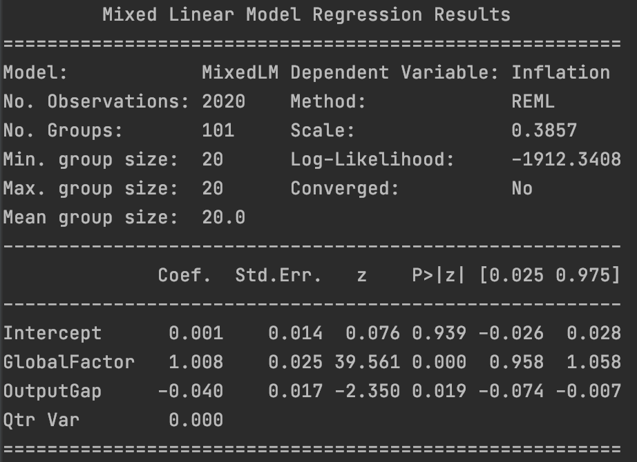
The panel regression estimates show that the slope of the global factor is indistinguishable from unity. Meanwhile, the output gap is significant and bears the right sign, although the effect size is very small. So, as a first pass, we can think of domestic slack as having a second order effect on domestic inflation in the advanced economies which is otherwise governed by a single global factor that captures slack in the global production system.
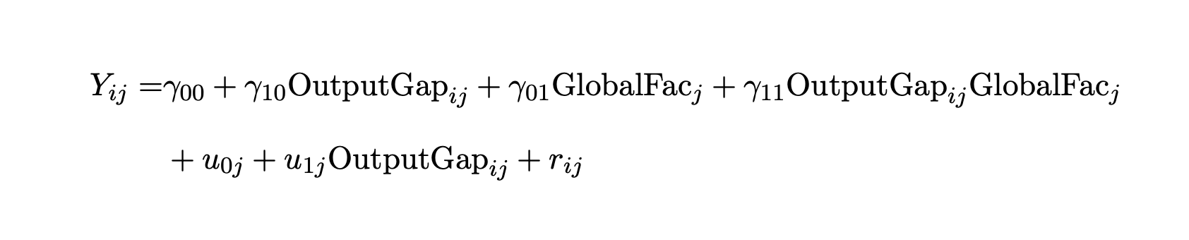
In the general setting of hierarchical modeling, we have a top-level model that relates a response to features of interest, stratified by a grouping variable. The coefficients of the top-level model are allowed to vary by group. In the general linear formulation, Y is a linear function of X within each group j, but the intercepts and the slopes are themselves functions of W, a variable that varies across groups indexed by j as below:
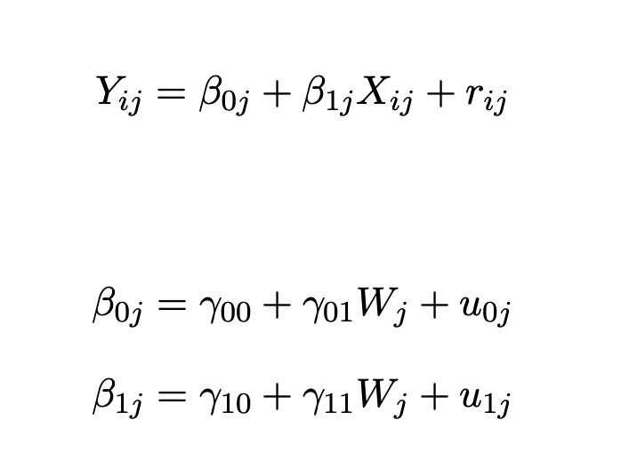
where the error terms are assumed to be homoskedastic and orthogonal to each other (except for the second level where it is possible to admit correlated errors). These equations cannot be estimated by ordinary least squares. But they can reformulated as a mixed-effects model and thereby estimated with suitable algorithms. Specifically, the equations above can be combined to yield the mixed-effects model:
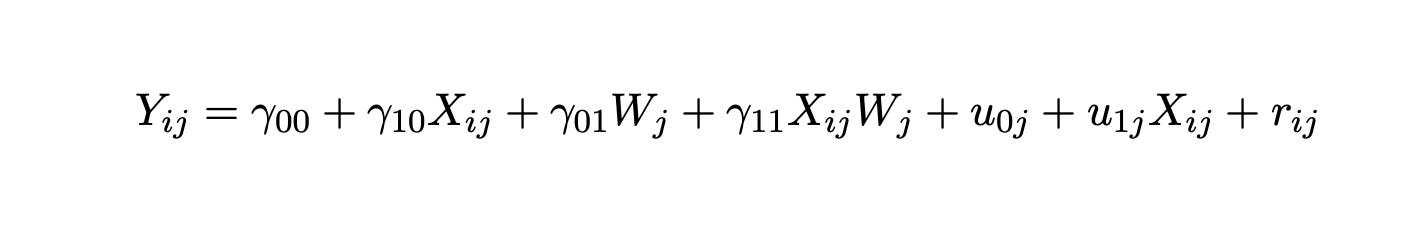
where we stratify by groups indexed by j. The first four terms are the fixed-effects; while the last is an idiosyncratic error term and the two terms preceding it are the random-effects. The magical thing about this methodology is that the second level parameters of the general hierarchical model can be recovered from the fixed-effects.
Given this general methodology, we propose the following hierarchical model of inflation in the advanced economies. At the top level, we retain the Standard Model — inflation is modeled as a linear function of the domestic output gap. However, we stratify by quarter, and allow the intercepts and slopes of the Standard Model to vary as a function of the global factor. The interpretation is that the responsiveness of inflation to the output gap depends on global conditions, which we proxy by our global factor — mean AE inflation.
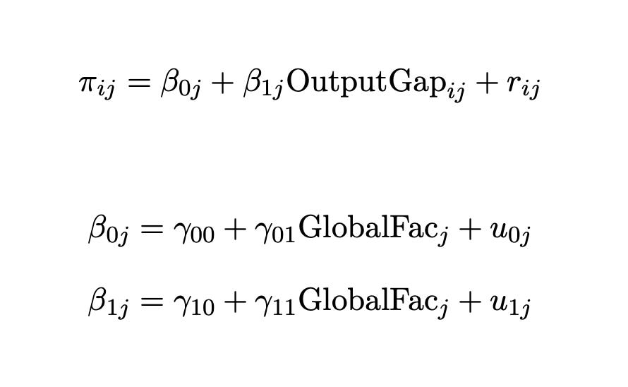
We may then estimate our hierarchical model from the following mixed-effects model:
The interpretation of the fixed-effects of the above mixed-effects model is clear from our two-level hierarchical model. Essentially, what we have is a Phillips curve with time-varying coefficients. Our estimated model is displayed below:
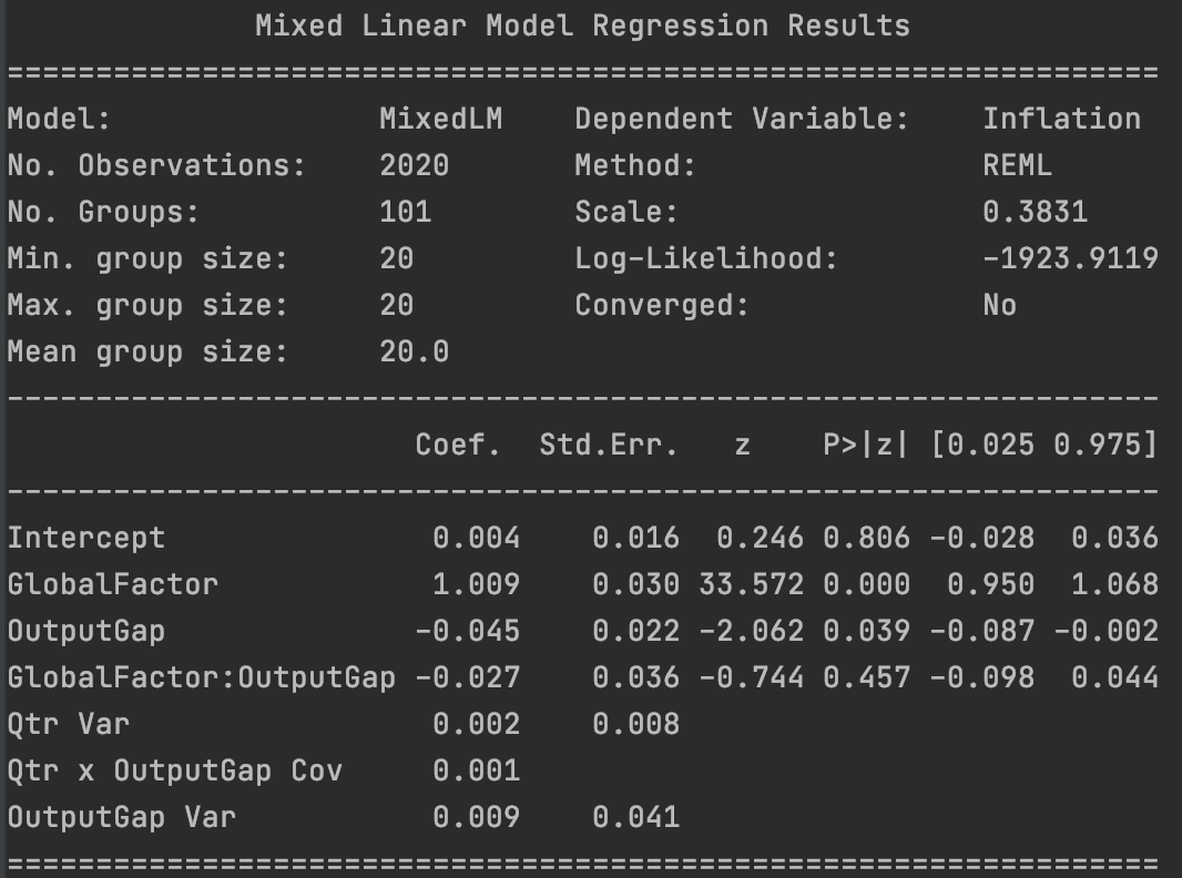
The intercept of the time-varying intercept of the Phillips curve, gamma(0, 0) is statistically indistinguishable from zero. However, the slope of the time-varying intercept of the Phillips curve, gamma(0, 1) equals 1.009 with a standard error of just 0.030. This means that the intercept of the Phillips curve is basically the global factor.
Meanwhile, the intercept of the time-varying slope of the Phillips curve, gamma(1, 0) equals -0.045 with a standard error of 0.022. So it is significant at the 5 percent level and bears the right sign. But the slope of the time-varying Phillips curve vanishes: gamma(1, 1) equals -0.027 with a standard error of 0.036.
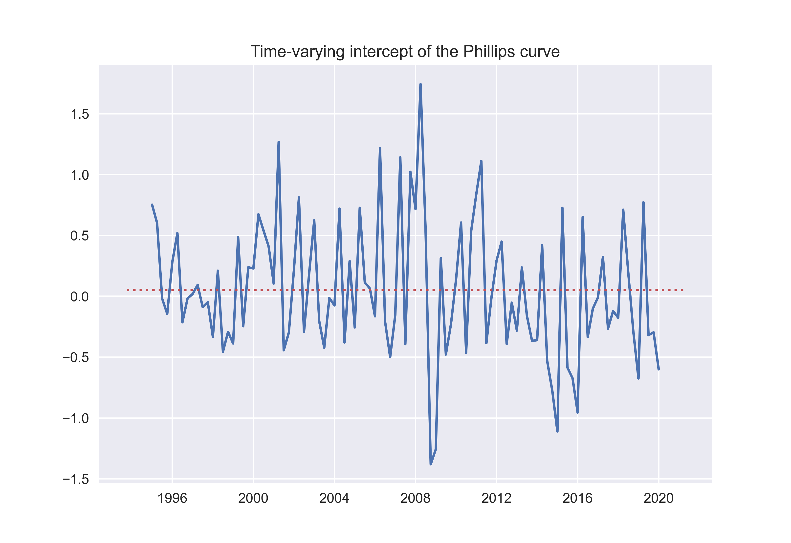
The next figure displays the time-varying intercept of the Phillips curve that we have seen is simply the global factor:
And the next figure displays the time-varying slope of the Phillips curve.
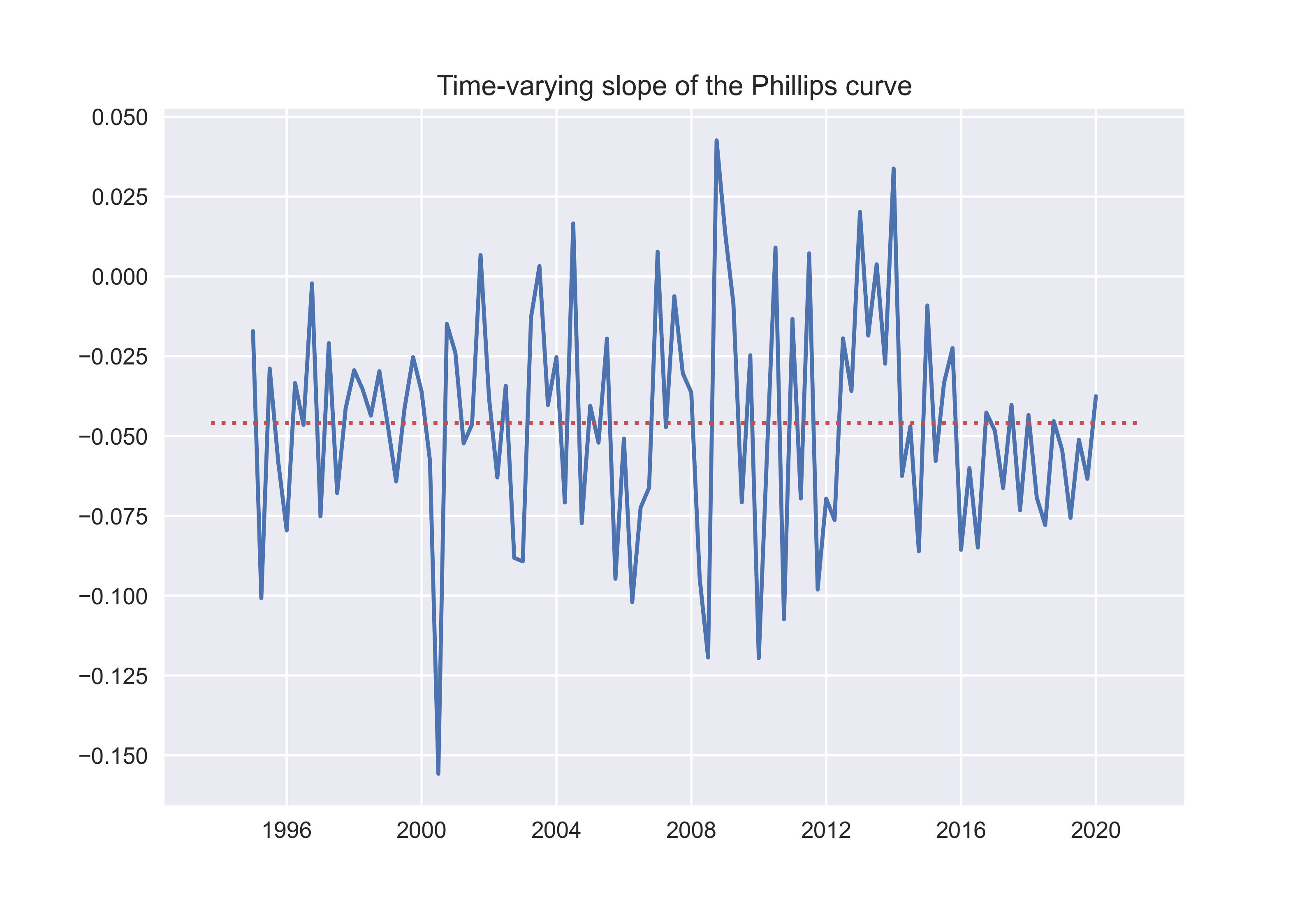
The two series look stationary. The augmented Dickey-Fuller test reveals that they are indeed.
Given these estimates, we have the following reduced-form model of inflation in the center countries:
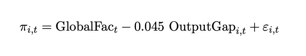
This is precisely the model suggested by the panel estimate we began with. Inflation in the advanced economies is given by a single global factor and a second-order correction term associated with the domestic output gap. This is what has become of the Phillips curve under the intensified global condition.